data markets post-thesis I: online regression

TLDR

• This post is about online regression in varying feature spaces
• We construct two models for this use case, OLM and OLM-S
• We compare to current literature on online classification in varying feature space
• And then move on to regression
• We do all this so we can use it in my next post (COMING SOON) to construct online regression markets in varying feature spaces

Hi! I originally started writing this blog post while I was writing my thesis. However, writing a thesis turned out to take a lot of time and effort - and somehow, one more writing project was not the highest on my list. Now, I handed in my thesis and took the time I needed away from the project.

My thesis was titled "Online regression markets with varying feature space". In one sentence, it concerns trading data using the regression market approach in situations where the available set of features changes over time. That sounds complicated but let's break down the keywords, ordered by importance:

1. Markets - people are trading something, in this case they are trading data for use in regressions
2. Regression - Using data to train predictive models and making predictions with those models on new data
3. Online - Referring to the fact that we're using online regression, which is regression where the regressor is continuously updated as new information becomes available (see my last blog post)
4. Varying feature spaces - Usually regression is done on a fixed set of features. In my thesis, however, I let the set of features change over time, with several implications regarding both markets and regression problems.

I am going to semi-cleanly split the results into two posts. This first part will be about online regression, or in fact supervised online learning in general, with varying features over time. The second part will be about the implications of varying features for data markets. Online learning with varying features over time turns out to already have a name in literature, known as Utilitarian Online Learning.

utilitarian online learning

Utilitarian Online Learning is a term first coined in a survey article from 2023³. It refers to machine learning that fulfills three criteria:

1. It's online - The model is updated continuously as new data becomes available
2. It natively handles varying feature spaces, i.e. it works just fine if the set of features available changes over time, and it might at one time step receive five features and at the next time step receive eleven other features, and it'll be fine with that.
3. It's computationally pretty fast

The third criterion is there to avoid lumping in things like retraining a batch regression mechanism at every time step using only the features present at that time step. While that is indeed a kind of online learning, and it does natively handle varying features, it's computationally VERY expensive, so it's only rarely useful in the situations utilitarian online learning models are intended for.

The survey article includes comparisons of a few algorithms for classification tasks. I readily decided to use the OCDS algorithm initially from the paper He et al. (2019)⁴, since it is fairly simple and seemed to be easily converted to a regression mechanism, if needed. I then tried implementing the OCDS algorithm myself, so that I could compare its results to my own.

issues with OCDS

As I started implementing OCDS, I ran into some confusion with the data in the original OCDS paper. I also didn't manage to reproduce the results of that paper despite several attempts. Unfortunately the authors of the OCDS paper could not share the code that generated their results since it was undergoing a patenting process. Therefore, I skipped on using OCDS and only compared to its results. I only discuss this slightly more in the results section, but if anyone involved in OCDS wants to tell me what's going on, that would be super welcome :)

my own models

As I realized I couldn't use OCDS, I decided to implement some models of my own. I developed two models, and they are both based on pretty simple concepts. Both are essentially based on linear regression.

Linear regression is essentially an optimization problem; we have a set of observations X and a set of targets y, and we're then looking for the coefficients a that gets the value of \(AX\) as close as possible to \(y\), measured by the square difference. Mathematically, this can be expressed as

$$ \underset{a}{min} \sum_i^N (a \cdot x_i - y_i)^2 $$

Here, i understand \(a\) as a vector of coefficients, \(y\) as a vector, and \(X\) as a matrix. \(x_i\) is a single row of the matrix \(X\), and there are \(N\) total rows. The optimum point of this optimization problem can be found analytically. You can transpose some matrices, multiply some matrices together, and then invert some things, and you get the analytically optimal vector of coefficients \(a\). I've referred before to this blog post which I think is great if you're interested in the basics of linear regression.

It can however also be solved in another way, which you have probably heard of before. If you think of the sum as a function of \(a\), \(\Phi(a) = \sum_i^N (a \cdot x_i - y_i)^2 \), you can follow the gradient of the function \(\nabla_a \Phi(a) \) backwards towards the minimum of the function. In essence, you look at the error locally and update \(a\) to minimize the error. This is known as gradient descent, which is the method neural networks also use to update their coefficients (a.k.a weights).

For the linear regression problem above, we would take the gradient with regards to the coefficients \(a\), i.e.

$$ \nabla_a \sum_i^N (a \cdot x_i - y_i )^2 = 2 x_i(a \cdot x_i - y_i) $$

From here on out I'll refer to the objective function as \(\Phi\), so we minimize \(\Phi\) and can then refer to the gradient as \(\nabla_a \Phi\). To solve the problem for the optimal parameters \(a^*\), we can then iteratively update our estimate, which we'll denote \(\hat a_t\) at a given time step t, by following the gradient. We then get an update step

$$ \hat a_{t+1} = \hat a_t - \tau \nabla_a \Phi $$

Where \(\tau\) is a step size. We're just going to use fixed step sizes, but one could feasibly reduce this step size over time. In fact, for any convex problem, reducing step sizes according to some specific rules will guarantee convergence.

Now we can iteratively walk towards the optimum by following the gradient. Right now we calculate the gradient based on the entire dataset, but what if we instead only took a subset of the dataset at every time step, and calculating the gradient based on just that? This will in fact also converge to the optimum solution, under some conditions, and is known as stochastic gradient descent. We can do this using just a single row of the dataset, or observation, at a time - and now we might see how we can create an iteratively updating model that updates as new information comes in. We update the model at every time step using that new information to calculate our gradient. This is the core method of the two online models I have developed.

online linear model (OLM)

So now, we know the central concept of updating an online model using stochastic gradient descent. Let's look at how exactly a linear regression model would look if it were to learn iteratively from observations that come in one at a time, using stochastic gradient descent for its update.

So, at time step \(t\), we receive the data point composed of features \(x_t\) and true label \(y_t\). When we come to this time step, we have an estimate of our coefficients \(\hat a_t\), and we can then produce an estimate of the true label \(\hat y_t\). Our gradient based on this single time step will be

$$ \nabla_{\hat a} \Phi_t = \nabla_{\hat a} (\hat a_t x_t - y_t)^2 = 2x_t(\hat a_t x_t - y_t) = 2 x_t(\hat y_t - y_t) $$

We then have the pretty simple update step of

$$ \hat a_{t+1} = \hat a_t - \tau 2 x_t (\hat y_t - y_t) $$

This gives us a linear regression model that we can use in an online fashion, i.e. updating it every time we get new observations. That's not quite enough for our Online Linear Model (OLM), though, since it also needs to handle missing features.

Usually when performing regression, we'll normalize our features so that they have a mean of zero. This mean is also the expected value of any feature absent of other information. When a feature is missing, the simplest way to handle it is to assume that the feature has the value of its mean, known as mean imputation. Then, if we always normalize input features for this model, we can just set missing features to zero. Then its term in the sum determining \(\hat y\) becomes zero, its term in the gradient becomes zero, and computationally we can just ignore it.

Then, we have an online linear regression model that can handle missing features, using the following steps at each iteration:

1. Get observation \(x_t\)
2. Ignore any missing features; initialize coefficients of previously unseen features to zero.
3. Calculate predicted value \(\hat y_t\) based on current coefficent vector \(\hat a_t\)
4. Calculate updated coefficient estimates based on true label \(y_t\) using gradient \(\nabla_{\hat a} \Phi = 2 x_t(\hat y_t - y_t) \)

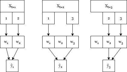
Below is a figure representing the behavior of predicting and fitting the OLM model for three time steps. It shows how features are only used when they are present, and the weights are also only updated when the features are present, then.

online linear model with subregressions (OLM-S)

The Online Linear Model just handles missing features by mean imputation. This is not very informative, and we have all of these other features lying around that might be correlated with the feature we're missing. This model instead reconstructs missing features using another level of online linear regression models.

So basically, at every time step where a given feature is present, an online linear regression model is fitted using that feature as the target and the rest of the features as features. It's kind of like every feature has an associated sub-model, or subregression, hence the name. I've demonstrated the overall concept below:

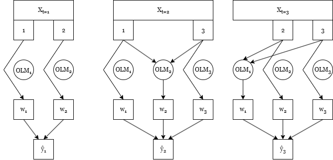
Here, we see how features are used for prediction. On the other hand, for fitting, all the present features have their subregressions using themselves as a target whenever they are present. As an example, below are explanations for what happens with feature two at every time step in the above example:

1. Features 1 and 2 are present at this time step. An OLM model with feature 2 as the target is initialized, and it is trained using feature 1 as the features and feature 2 as the target.
2. Feature 2 is now missing, but feature 1 and 3 are present. Feature 3 has never been seen before by the OLM model for feature 2, so it has its coefficient initialized to zero. Then, feature 2 is reconstructed using only feature 1, and the reconstructed feature 2 is passed along with feature 1 and 3 to the overall regression.
3. Feature 1 is missing, but feature 2 and 3 present. Feature 2 is then not reconstructed, but its subregression is trained using feature 2 as a target and feature 3 as a feature.

The update steps for each online linear model are then the same as before for the OLM.

modifications for classification

So far, we've only looked at least-squares regression problems. However, OCDS is a classification method, so I also want to look at the performance of these models for classification. Luckily, we can pretty easily convert these models to classification using the approach of Logistic Regression. This approach applies a nonlinear activation function on the output of the model known as the logistic function or Sigmoid function, \( h(x)=\frac{1}{1+e^{-x}} \). This function essentially views the input as the logarithm of an odds ratio, and converts log-odds to probability. Any real number is a valid log-odds ratio, so it's essentially a way to convert any number on the real number line to a probability between 0 and 1. The predicted probability of the model is then \( \hat y = h(a \cdot x) \), and the predicted label is 1 if \(\hat y > 0.5\), or 0 if \( \hat y < 0.5 \). The minimized loss function is Binary Cross-Entropy (BCE),

$$ \Phi = \sum_t (y_t \log(\hat y_t) + (1 - y_t) \log(1-\hat y_t)) $$

BCE comes from the log-likelihood function of the Bernoulli distribution. Basically, it comes from assuming that every true label \(y\) comes from a distribution where it has probability \(\hat y\) of being 1 and \(1-\hat y\) of being 0. That's a very surface-level understanding, but otherwise check out this Stanford pdf or this PennState lesson. This is to say that BCE is well founded, and based on Maximum Likelihood Estimation.

This combination of loss function and nonlinear activation function happens to give an extremely simple single time step gradient of

$$ \nabla_a \Phi = x_t (\hat y_t - y_t) $$

Which happens to be almost identical to the gradient of the parameters for linear regression expressed in \(x_t\), \(\hat y_t\), and \(y_t\), except for a power of two. The fact that the gradient turns out simple and easily calculable is a big reason why the sigmoid function is so often chosen for the final activation function of neural classification models.

classification results

Since the models in the literature are mostly classification models, I first tested my models on classification problems to test their performance compared to the models found in the survey article. The tests simulate the core problems these models are intended for, i.e. receiving data in an online fashion with some amount of missing data that randomly changes every time step. The pseudocode for running an online model shown below:

The specific test we will make will use datasets from the UCI databank¹. Every time step will have 50% of data removed by random choice.

Apart from testing my models and the models from the survey article, I also found a theoretical maximum accuracy for these models. This theoretic maximum is the accuracy of a logistic regression model, but trained insample on the dataset with no observations removed. I.e., where other models must iteratively predict and improve their coefficients one step at a time, this model is trained on the entire dataset \(X\) with no missing data, before then predicting on the entire dataset to create the full prediction vector \(\hat y\). The model will thus basically maximize accuracy.². I denote this model 'Logistic UB' for Upper Bound.

I've put the results from my models and the models from literature in the table below. Note that there are two reported values for OCDS, one from the OCDS paper itself, and one from my reimplementation of OCDS. The OLVF paper doesn't report results for all the used datasets, which is why some cells have N/A. I've marked the best performing model in bold, ignoring the OCDS paper results for reasons that will become apparent, and the insample optimal model for reasons I hope are obvious

Mean Accuracy	OCDS (paper)	OLVF	OVFM	OCDS (mine)	OLM	OLM-S	Logistic UB
australian	0.886	N/A	0.783	0.753	0.767	0.768	0.858
ionosphere	0.906	0.774	0.752	0.748	0.795	0.787	0.937
german	0.827	0.649	0.681	0.701	0.705	0.709	0.755
wdbc	0.951	0.903	0.918	0.921	0.938	0.935	0.993
wbc	0.939	0.913	0.922	0.934	0.938	0.941	0.961
magic04	0.886	0.644	0.762	0.732	0.732	0.743	0.791
kr-vs-kp	0.912	N/A	0.687	0.733	0.750	0.753	0.960
credit-a	0.926	N/A	0.760	0.766	0.783	0.780	0.864

(sorry, people on mobile) Okay, so what do we notice?

1. The OLM and OLM-S models are performing super well, OVFM is only occasionally better.
2. except for OCDS, which reports way higher results. However, OCDS also outperforms the theoretical optimum insample predictor.
3. OLM and OLM-S are almost identical in performance.

I don't think it's possible for an online model learning iteratively to beat an insample trained logistic regression model, so I think the test method in the OCDS paper might have been different from the one I present and other papers use. I take these results as a good indication that OLM and OLM-S are really pretty good utilitarian online models, even though they are very simple. However, I also get the indication that the reconstruction step from OLM-S does not add anything to the classification accuracy.

I've only covered the 50% missing data case, and my results indicated that some of these other models were better at 75% missing data, but I don't want to bombard you guys with too many graphs and tables, so we'll leave classification at this.

regression results

None of the other methods have implemented a regression variant, so from here on out I can only compare OLM and OLM-S. I have two questions that I want to answer:

1. How does OLM and OLM-S compare? Does the OLM-S reconstruction step actually improve performance for regression?
2. How does the correlation between features affect the performance of these models?

I tested generally using the same process as before. However, I added another thing: When using online models, you can often know several features forwards in time without knowing the labels, e.g. you just received \(x_{55}\) for time step 55, but you only know \(y_{30}\). There are 25 time steps between the two, which I'll denote as a forecast horizon of 25. When testing the methods, I'll vary the forecast horizon.

My test data here is completely synthetic; \(X\) is multivariate gaussian noise, and \(y\) is then given as a linear function of \(X\) with coefficients \(\alpha\) and some added gaussian noise. Mathematically,

$$ x_t \sim \mathcal N (\mathbf 0, \Sigma) \, \forall t, \,\,\,\, y_t = \alpha \cdot x_t + \mathcal N(0, 1) \, \forall t $$

I parameterize the covariance matrix for \(X\) by a single parameter \(\rho\) less than 1 to control the correlation between features. The covariance matrix is given by \(\Sigma_{i,j} = \rho ^{\min(|i-j|, N-|i-j|)}\). This looks complicated, but it really isn't. It's a matrix where the covariance between two features is given by how far they are from each other, i.e. feature 2 and 4 will have a smaller covariance than feature 2 and 3. It is then forced to be symmetric, so if there's e.g. 5 features, the correlation between feature 0 and 1 is the same as between feature 0 and 4.

I tested on a synthetic dataset with 200 time steps. I used the MSE as my metric, since this is the loss function minimized by the regressors. I'll also set the forecast horizon to 25 time steps. I also created a regression variant of OCDS and included it as well.

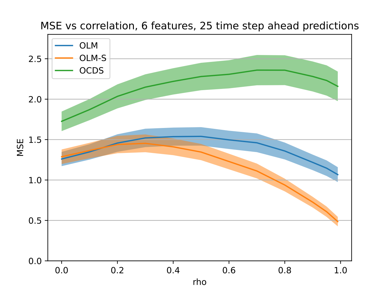
We see that OLM and OLM-S perform the same when correlations are low, but OLM-S starts outperforming OLM as the correlation increases. We see also that the reconstruction step of OLM-S really starts to improve forecasting accuracy once the correlation gets higher. That's a nice confirmation that it's even worth it to do, which it didn't seem to be for classification. OCDS doesn't perform well at any point.

I also tested different forecasting horizons using the same method, as shown below:

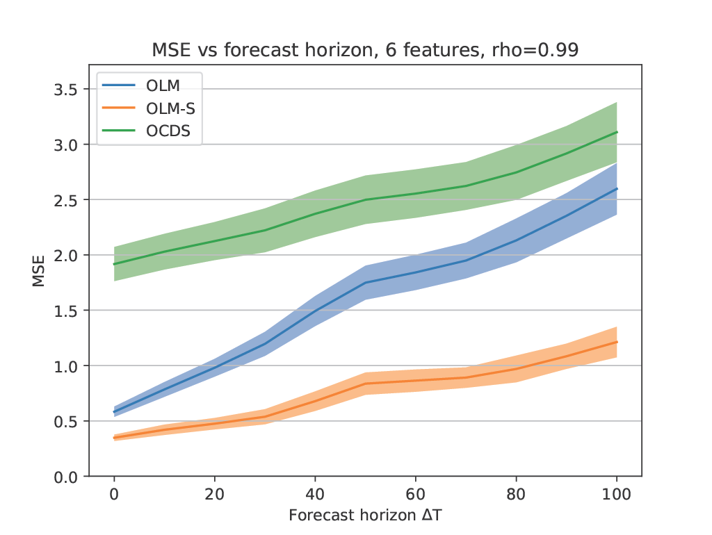
This is with a correlation of 0.99. We see that as the forecast horizon increases, OLM-S starts performing a lot better, indicating it can draw more information out of fewer observations.

So that is pretty cool. I am surprised there isn't more literature in this area for me to compare to. If anyone knows some other online regression methods for varying feature spaces I can test against, please let me know. I'd love to see how these size up. Note that for the next step, constructing fair markets based on these regression methods, I needed convex methods. This is why non-convex online regressors such as Mondrian forests were excluded.

From a computational complexity point-of-view, OLM computationally is linear in the number of features it sees \(n\), so of \(O(n) \), and OLM-S is quadratic, \(O(n^2) \). OCDS, on the other hand, has a cubed runtime \(O(n^3) \) in the general case, but has some optimizations to limit this in practice.

conclusion

Okay, now we've established some models that we can use for regression in an online fashion when the amount of available features varies freely in time. The existing literature didn't have any convex utilitarian online regression methods available, but we constructed two models, OLM and OLM-S, that are convex, online, and handle varying feature spaces.

This is everything I needed in terms of models for my thesis, and I could then move on to trying to construct data markets for this situation. We'll move on to that next time :)

references

¹ Specifically, the dataset UCI IDs are as follows: australian:143; ionosphere:52; german:144; wdbc:17; wbc:15; magic04:159; kr-vs-kp:22; credit-a:27.

² Actually, the accuracy is not necessarily maximized, see e.g. this stackexchange post. It is however a very good proxy.

³ Yi He, Christian Schreckenberger, Heiner Stuckenschmidt, and Xindong Wu. Towards utilitarian online learning - a review of online algorithms in open feature space. Ijcai International Joint Conference on Artificial Intelligence, 2023-:6647–6655, 2023. ISSN 10450823.

⁴ Yi He, Baijun Wu, Di Wu, Ege Beyazit, Sheng Chen, and Xindong Wu. Online learning from capricious data streams: A generative approach. Ijcai International Joint Conference on Artificial Intelligence, 2019-:2491–2497, 2019. ISSN 10450823. doi: 10.24963/ijcai.2019/346